The Master Theorem

Definition
Examples
- Binary Search
- Merge Sort
Informal Proof
Formal Proof

The Master Theorem is a common and important tool, used in the asymptotic analysis of algorithms: particularly recursive, divide-and-conquer algorithms, common examples of which include Binary Search, Merge Sort and Quick Sort.

Definition

Where $T(n)$ is the running time of an algorithm for an input size $n$, we define the upper bound with:

\[ T(n) \leq c \quad \forall \quad \text{sufficiently small $n$} \]

otherwise,

\[ T(n) \leq a T\left(\frac{n}{b}\right) + O(n^{d}) \]

where:

$a$ is the number of times the algorithm is recursively called per (non-final) call.
$b$ is the factor by which the problem size decreases per recursive call.
$c$ is a constant for the running time of the base case. It is not used in the theorem.
$d$ is the power of the running time of the "main part" of the algorithm. What is meant by this will be made clear in the examples.

Once we have these values defined, the master theorem is simply that the running time of the algorithm is:

\[ T(n) \leq \begin{cases} O(n^d \log n), & \text{if } a = b^d \newline O(n^d), & \text{if } a < b^d \newline O(n^{\log_b(a)}), & \text{if } a > b^d \end{cases} \]

Examples

Binary Search

The Binary Search algorithm is supplied a sorted array of length $n$, compares the middle element to the one it is searching for, then based off those makes a recursive call on either the left or right half of the array, until the element it is searching for is found, or the size of the array is one and the element is not present.

The below pseudocode is not complete, however it should provide an idea of how Binary Search works, if you are not already familiar with it.

def BinarySearch(int array[N] A, int target):
    if array[N/2] == target:
        return True
    left = left half of A
    right = right half of A
    if array[N/2] > target:
        return BinarySearch(left, target)
    if array[N/2] < target:
        return BinarySearch(right, target)

We see that BinarySearch only calls itself once - there are two possible places, however in one call, only one of them can be called: this means $a = 1$.
As recursive calls only look at one half of the given array, we see that $b = 2$.
The work done by the algorithm not recursively is just a comparison, which runs in constant time, so $d = 0$.

$b^d = 1 = a$, so we refer to the first case, and find that the running time of binary search is $O(\log n)$, which matches what we already know about Binary Search.

Merge Sort

The Merge Sort algorithm is supplied an unsorted array of length $n$, then recursively sorts sub-arrays, then merges them into larger arrays. If you haven't encountered this algorithm before, this concept may take a little while to get your head around: below is some pseudocode that may help.

def MergeSort(int array[N] A):
    if N == 1:
        return A
    sorted_left = MergeSort(left half of A)
    sorted_right = MergeSort(right half of A)
    i, j = 0
    sorted_array = []
    while True:
        if i == len(sorted_left):
            sorted_array.append(rest of sorted_right)
            break
        if j == len(sorted_right):
            sorted_array.append(rest of sorted_left)
            break
        if sorted_left[i] < sorted_right[j]:
            sorted_array.append(sorted_left[i])
            i++
        if sorted_right[j] < sorted_left[i]:
            sorted_array.append(sorted_right[j])
            j++
    return sorted_array

The part that is done recursively, is obtaining the sorted left and right halves. What the algorithm does not do recursively however is merge the two halves to make one larger sorted array.

Recursively, we make 2 calls, for the sorted left and right halves, so $a = 2$.
Each recursive call receives a problem of half the size, so $b = 2$.
The running time of the merge at the end of the call is $O(n)$, so $d = 1$.

$b^d = 2 = a$, so we use the first case again: the running time of Merge Sort is $O(n \log n)$, which matches what we should know.

Quick Sort is a slightly interesting case as its worst case scenario is actually $O(n^2)$ (think about going through it on a sorted array). However, assuming an optimal quicksort - meaning it always takes the median element - you should now be able to prove that it has $O(n \log n)$ performance.

Informal Proof

I call this a "proof", because really we only want to build some intuition about the working of the master theorem rather than to build a formal proof.

There are 3 cases to consider, which we will try to cover one-by-one:

The case where all the nodes have equal work to do.
The case where child nodes have less work to do.
The case where child nodes have more work to do.

When all the nodes have equal work to do, we mean that the amount of work is the same at every recursion level. The amount of work per level is $n^d$ and there are $\log n$ levels, so we can intuitively say that in this case there is a total of $O(n^d \log n)$ work being done.

When the child nodes have less work to do, we can expect that most of the work is being done at the top of the recursion tree. This means that the most significant amount of work is that which is done at the root, not recursively: this means an $O(n^d)$ complexity.

Conversely, when the child nodes have more work to do, we can expect that most of the work is being pushed onto the leaf nodes. However, at the leaf nodes, we are at the base case, so the complexity for each individual one is in constant time: this means the overall complexity is just the number of leaves: $O(\text{no. leaves})$. So what's the equation for the number of leaves? The equation for the number of leaves is the number of sub-calls per sub-call (i.e. the rate of proliferation) to the power of the number of levels: $a^{\log_b(n)}$. As seen below, this is the same as $n^{\log_b(a)}$.

Using the $\log(x^w) = w \log x$ rule of logarithms:

\[ \log_b(n)\log_b(a) = \log_b(a)\log_b(n) \]

\[ \log_b(a^{\log_b(n)}) = \log_b(n^{\log_b(a)}) \]

\[ a^{\log_b(n)} = n^{\log_b(a)} \]

Formal Proof

Consider this in the form of a recursion tree, the below one should make this easier. Here specifically we have the case of $a=2$.

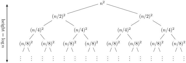
Figure 1: recursion tree where a=2

There are $log_b n + 1$ levels in the tree, and where $j$ is the level the tree is on, each subproblem is of the size $\frac{n}{b^j}$; furthermore, it will take at most $c\left(\frac{n}{b^j}\right)^d$ work to solve. There are $a^j$ subproblems on each level, so on each level there is a total of $a^j \cdot c \cdot \left(\frac{n}{b^j}\right)^d = cn^d\left(\frac{a}{b^d}\right)^j$ work being done on each level.

This means that the total amount of work being done is

\[ cn^d \sum^{\log_b n}_{j=0} \left(\frac{a}{b^d}\right)^j \]

So now there are 3 cases to consider:

The case where $a = b^d$
The case where $a < b^d$
The case where $a > b^d$

When $a = b^d$, we know that $\frac{a}{b^d} = 1$, so the amount of work being done is: \[ cn^d \sum^{\log_b n}_{j=0} 1 = cn^d \log_b n \in O(n^d \log n) \]

When $a < b^d$, we know that $0 < \frac{a}{b^d} < 1$, so we know that the sum converges to a constant.

\[ \sum^{\log_b n}_{j=0} \left(\frac{a}{b^d}\right)^j \leq \sum^{\infty}_{j=0} \left(\frac{a}{b^d}\right)^j = \frac{1}{1 - \frac{a}{b^d}} \]

So the sum for the total work being done is less than or equal to some constant (as $a, b, d$ are all constants).

It follows that in the case $a < b^d$:

\[ cn^d \sum^{\log_b n}_{j=0} \left(\frac{a}{b^d}\right)^j = cn^d k \in O(n^d) \]

Where $k$ is a constant $\leq \frac{1}{1 - \frac{a}{b^d}}$.

The final case to prove is the case where $a > b^d$:

\[ \sum^{\log_b n}_{j=0} \left(\frac{a}{b^d}\right)^j = \frac{1 - \left(\frac{a}{b^d}\right)^{\log_b n + 1}}{1 - \frac{a}{b^d}} \]

$a, b, d$ are constants, so we find this is in $O\left(\left(\frac{a}{b^d}\right)^{\log_b n}\right)$.

We have already established that $a^{\log_b n} = n^{\log_b a}$. We can use the same method to show that $b^{d\log_b n} = n^{d\log_b b} = n^d$.

This means that our total work done in this case is

\[ cn^d \sum^{\log_b n}_{j=0} \left(\frac{a}{b^d}\right)^j \in O\left(n^d \cdot \frac{n^{\log_b a}}{n^d}\right) = O(n^{\log_b a}) \]

So we have now proven all three cases of the master theorem.